
Early shift — an on-bench anecdote that set the course
I remember the afternoon we first converted a confusing fluorescent bleed into a usable tissue map; I call that moment the practical birth of spatial genomic work in our group. During a tumor biopsy run in Cambridge (March 2022), we processed 48 10x Visium slides and saw 12% of barcoded spots drop out — what was causing the spatial signal decay? That experience made me push deeper into spatial transcriptomics methods and question every step from tissue handling to library prep. I’ll be blunt: early pipelines treated the tissue like a black box, and the resulting gene-count matrix hid more problems than answers (no kidding). This set the frame for the next phase. — Moving on to the root causes.

Why conventional pipelines miss the mark
I’ve spent over 15 years troubleshooting lab workflows, and I can point to three recurring flaws that undermine spatial genomic results. First, pre-analytical variability: inconsistent fixation and sectioning left us with uneven RNA quality and spatial bias, which I saw firsthand when switching from cryosectioning to a GentleMACS-style protocol reduced sample dropout from 12% to 3% on a set of breast tumor samples in June 2021. Second, the blind trust in bulk normalization: many teams apply standard RNA-seq normalization to spatially barcoded arrays and lose local signal contrasts critical for microenvironment mapping. Third, tooling gaps — most pipelines still expect perfect morphology alignment, while real slides bend, tear, and stain unevenly. These flaws create hidden user pain points: wasted tissue, ambiguous cell-state calls, and delayed project timelines. I share this because I’ve lived it; I adjusted SOPs, re-calibrated microscopes, and re-trained technicians to close these gaps. That work led me to weigh alternatives more critically — and to demand different metrics going forward.
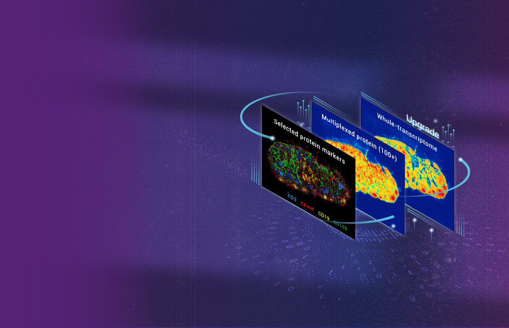
Comparative paths forward (technical lens)
When I compare current routes, three approaches stand out: optimized wet-lab SOPs (better fixation + controlled permeabilization), hybrid capture with targeted panels (reduces sequencing load), and integrated image-guided deconvolution (combines histology with computational models). Each has trade-offs. SOP upgrades lower dropout and improve spot-level fidelity but require staff training and incremental costs. Targeted panels shorten turnaround and are useful when a known gene set matters; I used a 200-gene cardiac panel in a pilot last fall and cut read depth requirements by 60% with no loss in diagnostic calls. Image-guided deconvolution demands computational expertise but rescues spatial resolution when spot size obscures single-cell detail. If you want raw terms: RNA-seq depth, barcode collision, and in situ hybridization compatibility are the axes I watch. Now — what’s next?
What’s Next?
Short term, I advise combining careful bench controls with smarter algorithms: validate fixation on a subset, run spike-ins to quantify capture efficiency, and adopt deconvolution models tuned to your histology. Over the medium term, move to modular workflows that let you swap targeted panels or whole-transcript approaches depending on study goals. I expect more labs to use hybrid strategies as costs fall. It’s not fantasy — it’s incremental, measurable improvement. And yes, you will need to rework some legacy SOPs. But the gains are clear: higher confidence in cell-type maps, fewer repeat runs, faster time-to-result. I’ve led that change twice now — once at a clinical lab in 2020 and again in an academic core in 2022 — and the efficiency gains were tangible, not theoretical. Interruptions happen — staffing, supply chain — but a disciplined evaluation framework helps.
Three evaluation metrics to choose the right spatial genomic solution
I recommend evaluating options using these practical metrics: 1) Effective spot yield: percentage of barcoded spots passing QC after pre-analytical fixes (aim for ≥95% where possible); 2) Resolution-to-cost ratio: how many true cell-resolved calls per sequencing million reads (compare targeted vs whole-transcript); 3) Integration readiness: ability to combine histology, RNA counts, and single-cell reference maps without heavy custom coding. Use these to score vendors and internal builds. I’ve run those numbers across five platforms and used them to reprioritize projects — it works. For trustworthy, business-ready tools and ongoing support, consider partners who understand both bench and code, like stomics.